Banging a black hole

Everything vibrates. Not only do atoms and general quantum systems have characteristic frequencies, but spacetime itself vibrates. Propagating vibrations of spacetime are called gravitational waves.

You are a function of what the whole universe is doing in the same way that a wave is a function of what the whole ocean is doing.

Alan Watts

In a previous post, I gave a technical guide on how to solve wave equations on unbounded domains. The example was simple: the homogeneous, one-dimensional wave equation. While that’s a nice little toy problem, it’s too simple. The general solution can be written down explicitly; you don’t need numerics to solve it.

This post is about a more interesting problem: gravitational waves from black holes. This sounds cool, and it is. I’ll show you that computing gravitational waves is not that different from computing simple waves¹. All you need is an additional potential term. If you want to try it out, and numerically generate your own gravitational waves, you can run the code in Colab.

We will compute gravitational waves propagating in the spacetime of a black hole by solving the Regge-Wheeler-Zerilli equation \eqref{1}.

Black hole

First, a little pedantry. In general relativity, a black hole is actually not a “thing.” You may hear that it’s a collapsed, dense star. This is how it forms but it’s not the right way to think about it in classical relativity. As far as we are concerned, the black hole is a boundary of our domain². When I write about gravitational waves from a black hole, I don’t mean that the black hole is waving. What’s waving is the spacetime around the black hole. Avoid thinking of the black hole as “an object in space.” Instead, think of it as a boundary of your domain.

A black hole is rigorously defined as the region of spacetime from which no signal can escape to the outside universe where we are. The “surface” of a black hole, called the event horizon, marks the boundary of that region. The black hole’s interior is no longer in causal contact with the external universe. It is literally not part of the manifold in which external physics takes place³.

A black hole is not a hole in the usual sense⁴, and it’s not even black⁵.

Rockbiter: Near my home, there used to be a beautiful lake. But then… then it… it was gone.
Teeny Weeny: Did the lake dry up?
Rockbiter: No. It just wasn’t there anymore. Nothing was there anymore. Not even a dried up lake.
Teeny Weeny: A hole?
Rockbiter: A hole would be something. No, it was… nothing.

— The NeverEnding Story (1984)

The simplest black hole solution to Einstein’s equations was discovered, amidst heavy artillery fire and freezing conditions, a few months after Einstein published his equations for gravity. The Schwarzschild solution (in Droste coordinates) is given by the metric $$ ds^2 = - f(r) dt^2 + \frac{1}{f(r)} dr^2 + r^2 d\sigma^2, $$ where $d\sigma^2 = d\theta^2 + \sin^2\theta \ d\phi^2$ is the metric on the unit sphere and $$ f(r) = 1-\frac{2M}{r}, $$ with $M$ the mass of the black hole in natural units ($G=c=1$). Note how the function $f(r)$ vanishes at $r=2M$ leading to an apparently singular metric. This is the magic sphere (in Eddington’s words) that caused a lot of confusion in the early days of relativity. We now know that this singularity is an artefact of a bad choice of time. Our regular idea of time relies on the possibility of two-way synchronization. Such a construction is not possible at the event horizon because signals sent for synchronization inevitably vanish. We’ll fix this later; let’s first tickle this monster and see how it laughs.

Banging

We now perturb this spacetime⁶ by adding a small scalar, electromagnetic, or gravitational field. Scalar fields are simplest to demonstrate the basic features of wave propagation in black hole spacetimes. Below is a simulation that I made a few years ago that shows what happens to such a scalar field when you bang the spacetime at a point some distance away from the black hole horizon⁷.

We won’t perform a three-dimensional simulation, yet. To simplify the coding, we take advantage of the spherical symmetry of the black hole and decompose the scalar perturbation in spherical harmonics: $$ U(t, r,\theta,\phi)=\sum_{\ell=0}^{\infty} \sum_{m=-\ell}^{\ell} u_{\ell m}(t,r) Y_{\ell m}(\theta,\phi). $$ Each mode, $u_{\ell m}$, satisfies a one-dimensional equation that looks like this: $$ \left(\partial_t^2 - \partial_{r_\ast}^2 + V_\ell(r_\ast) \right) u_{\ell m}(t, r_\ast) = S_{\ell m}(t,r_\ast). \tag{1}\label{1}$$ The coordinate $r_\ast$ is called the tortoise coordinate and is defined by $$ dr_\ast = \frac{dr}{f}, \quad \text{or} \quad \partial_{r_\ast} = f \partial_r.$$ Its domain is unbounded in both directions with $r_\ast\in(-\infty,\infty)$. A significant portion of research in black-hole perturbation theory consists in solving an equation of the type \eqref{1} for various potentials $V_\ell$ and sources $S_{\ell m}$. We’ll assume no sources for this post and omit the mode-dependence in the notation. In general, you can think of the perturbations sourced by particles representing, say, a stellar black hole orbiting in the spacetime of a galactic, supermassive black hole (extreme-mass-ratio inspiral). Yes, you can indeed model crazy things with a simple equation like that.

You can simply discretize and solve the equation \eqref{1} on a truncated domain but where’s the fun in that⁸. Let’s solve it on the full black-hole spacetime using hyperboloidal compactification. The general structure of the equation \eqref{1} is the same as the one-dimensional wave equation discussed previously. The main difference is the potential term that can represent different types of perturbations. In this post, we want to calculate gravitational waves, so we use the gravitational potential⁹ given as a function of the areal coordinate $r$ as: $$ V_{\ell}(r) = \frac{f(r)}{r^2} \left( \ell(\ell+1) - \frac{6M}{r} \right), \tag{2} \label{2} $$ where $\ell$ is the angular momentum number in the spherical harmonic decomposition. Note that the potential is given by the areal coordinate $r$ but the wave equation is written in the tortoise coordinate $r_\ast$. We’ll fix this problem in a little bit. Let’s first handle the unbounded domain in the tortoise coordinate $r_\ast$.

Hyperboloidal compactification

To solve \eqref{1} on the infinite spacetime, we apply hyperboloidal compactification described in the previous post. The spatial compactification and the time transformation are $$ \rho = \rho(r_\ast), \qquad \tau = t + h(r_\ast), $$ We define $$ H_\ast(\rho):= \frac{dh}{dr_\ast}, \qquad G_\ast(\rho):= \frac{d\rho}{dr_\ast} = \left(\frac{d r_\ast}{d\rho}\right)^{-1}. $$ We write the wave equation \eqref{1} in symmetric hyperbolic form by defining auxiliary variables as before $$ \psi := \partial_\rho u, \qquad \pi := \frac{1-H_\ast^2}{G_\ast} \partial_\tau u - H_\ast \partial_\rho u. $$ The wave equation \eqref{1} becomes first-order symmetric hyperbolic $$ \begin{aligned} \partial_\tau u &= \frac{G_\ast}{1-H_\ast^2}\bigl(H_\ast \psi + \pi\bigr),\\[6pt] \partial_\tau \psi &= \partial_\rho \left[\frac{G_\ast}{1-H_\ast^2}\bigl(H_\ast\psi + \pi\bigr)\right],\\[6pt] \partial_\tau \pi &= \partial_\rho \left[\frac{G_\ast}{1-H_\ast^2}\bigl(\psi + H_\ast \pi\bigr)\right] {\color{red}+ \frac{V_\ell}{G_\ast} u}. \end{aligned} \tag{3}\label{3} $$ The only difference to the flat wave equation is the potential term in red. Since this is the main difference to the flat wave equation that allows us to compute gravitational waves from a black hole, let’s spend some time on it.

The gravitational potential

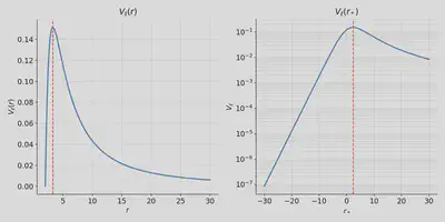
The asymptotic behavior of the potential \eqref{2} is determined by the factor $\frac{f}{r^2}$. The potential vanishes linearly at the event horizon and quadratically towards infinity. But by transforming to the tortoise coordinate we modify this behavior near the horizon because the tortoise coordinate diverges logarithmically as $r\to 2M$. Therefore, the potential \eqref{2}, or equivalently the term $\frac{f}{r^2}$, falls off exponentially toward the black-hole horizon and quadratically towards infinity in $r_\ast$. Below are two plots of the potential for $\ell=2$ and $M=\frac{1}{2}$, in $r$ and in $r_\ast$. The semilog plot in $r_\ast$ clearly shows the exponential decay on the left (near the horizon) and a quadratic decay on the right (toward infinity). The red dashed line marks the peak of the potential right outside the photon sphere around $r_p \approx 3.3 M$.

One of the reasons people like the tortoise coordinate, aside from the resulting familiarity of the equation \eqref{1}, is that it naturally provides increased resolution in the strong field region near the horizon. You can see this clearly in the right plot where the domain $r_\ast<0$ has no sharp gradients. Let’s think about this a bit in our setup.

In the compactified equation \eqref{3}, the gravitational potential is divided by the Jacobian $G_\ast$, which measures how the compactifying coordinate $\rho$ varies with the tortoise coordinate $r_\ast$. Since the infinite interval $r_\ast\in(-\infty, \infty)$ is mapped to a finite interval in $\rho$, we need $G_\ast\to 0$ at both ends. We must be careful that $G_\ast$ does not vanish faster than the potential for the ratio to be regular. Because the potential decays only quadratically towards infinity, we cannot use the exponential compactification from the previous post. In the exponential compactification, $G_\ast$ vanishes faster than $r^2$ grows and the potential term blows up. With $r_\ast = \mathrm{arctanh}(\rho)$ and $G_\ast=1-\rho^2$, and considering that asymptotically $r\sim r_\ast$, we get $$ G_\ast\ r^2 \sim (1-\rho^2) \ \mathrm{arctanh}^2\rho \to 0 \quad \text{as} \quad \rho\to 1. $$ The vanishing of $G_\ast r^2$ at infinity spoils regularity. Instead, we need an algebraic compactification. For example, something like $r_\ast = \tan\rho$ and $G_\ast=\cos^2\rho$, gives $$ G_\ast\ r^2 \sim \cos^2\rho \ \tan^2\rho = \sin^2\rho = 1 \quad \text{as} \quad \rho\to \frac{\pi}{2}. $$

There’s a geometric reason for this restriction in compactification. As $r\to\infty$ the surface area of spheres grow quadratically. Therefore, only an algebraic compactification leads to a regular equation. When we use a compactification that’s too fast, the potential blows up. When the compactification behaves algebraically, such as a trigonometric function, the limit is regular.

Having figured this out, why do we use $r_\ast$ in the first place? I mentioned that it gives us additional resolution near the horizon, but we’re compactifying. We can adjust it to get the resolution we need without going through the tortoise coordinate. Let’s get rid of it and compute the potential explicitly in terms of a simpler transformation $r(\rho)$. We just need to be careful about the Jacobian: $$ G_\ast = \frac{d\rho}{dr_\ast} = \frac{dr}{dr_\ast} \frac{d\rho}{dr} =: f G, $$ where we introduced $G:=d\rho/dr$. If we now consider $H_\ast$ also as a function of $r$ and transform directly to $\rho$, we can fully avoid the tortoise coordinate.

There are many possible radial compactifications. In Schwarzschild there is one particularly appealing choice: $$ \rho := f(r)=1-\frac{2M}{r} \implies r(\rho) = \frac{2M}{1-\rho}. $$ With this, the exterior domain $r\in(2M,\infty)$ is mapped to $\rho\in(0,1)$. The inner boundary at $\rho=0$ is the event horizon, $r=2M$, and the outer boundary at $\rho\to 1$ is infinity, $r\to\infty$. 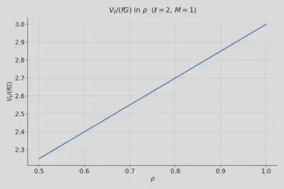The Jacobian reads $$G=\frac{d\rho}{dr} = \frac{d}{dr}\Bigl(1-\frac{2M}{r}\Bigr)=\frac{2M}{r^2} =\frac{(1-\rho)^2}{2M},$$ The rescaled potential term becomes $$ \frac{V_\ell}{G_\ast}=\frac{\ell(\ell+1)-3 (1-\rho)}{2M}. $$ This is beautiful! The potential varies only linearly with $\rho$. And the plot for $\ell=2, M=1$ is below.

Note that the compactification cancels the redshift factor $f$ from the original RWZ potential. And with this particular compactification, the rescaled potential is simply a linear function that barely varies over the entire domain. We’ll have no problem solving equations with such a simple term.

Time transformation

The final remaining ingredient for our system \eqref{3} is the boost $H_\ast$. Again, there are many choices. Arguably, the simplest choice that bridges the horizon and infinity is the minimal gauge. You can derive it by just requiring the proper behavior at both boundaries and regularity at infinity. Consider the $(t,r_\ast)$ block of the Schwarzschild metric: $$ ds^2_{t,r_\ast} = f \left(-dt^2 +dr_\ast^2\right). $$ In- and outgoing null rays of this metric are $v=t+r_\ast$ and $u=t-r_\ast$. We want the coordinate $\tau$ to behave as $v$ toward the horizon, and as $u$ towards infinity. This implies $H_\ast\to 1$ as $r\to 2M$ and $H_\ast\to -1$ as $r\to\infty$. Further, we want conformal regularity at infinity for the transformed metric: $$ ds^2_{\tau,r_\ast} = f \left(-d\tau^2 + 2 H_\ast d\tau dr_\ast + (1-H_\ast^2) dr_\ast^2\right). $$ Conformal regularity means a finite limit for $\Omega^2 ds^2$ when $\Omega\sim 1/r \to 0$. With compactification, we have $dr_\ast \sim \Omega^{-2}d\rho$. Therefore, the regularity of the radial component under conformal compactification implies: $$ 1-H_\ast^2 = (1-H_\ast) (1 + H_\ast) \sim \Omega^2 \sim \frac{1}{r^2}, $$ which means $$H_\ast = -1 + \frac{C}{r^2} + \mathcal{O}(r^{-3}), $$ as $r\to\infty$. These conditions are true for all time transformations bridging between the future event horizon and future null infinity. By omitting the lower order terms above, and imposing the requirement $H_\ast(r=2M)=1$ gives us the boost function for the minimal gauge: $$ H_\ast = -1 + \frac{8M^2}{r^2} = -1 + 2(1-\rho)^2. $$ In our compactifying coordinate $\rho$, the term that ensures the regularity of the compactified equation reads: $$ \frac{fG}{1-H_\ast^2} = \frac{1}{8M(2-\rho)}.$$ The minimal gauge leads to particularly simple expresions for the transformed system.

The numerical solution

Let’s wrap up. The choices for the compactification and time transformation above give us the following system \begin{equation} \begin{aligned} \partial_\tau u &= \frac{1}{8M(2-\rho)}\bigl(H_\ast\psi + \pi\bigr),\\[4pt] \partial_\tau \psi &= \partial_\rho\left[\frac{1}{8M(2-\rho)}\bigl(H_\ast\psi + \pi\bigr)\right],\\[4pt] \partial_\tau \pi &= \partial_\rho\left[\frac{1}{8M(2-\rho)}\bigl(\psi + H_\ast\pi\bigr)\right] +\frac{\ell(\ell+1) - 3(1-\rho)}{2M}u, \end{aligned} \end{equation} with $H_\ast=-1+2(1-\rho)^2$. The system doesn’t need any boundary data by construction. We simply apply one-sided stencils at the boundaries as before. All we need now is to prescribe some initial data (typically a localized Gaussian) and run the solver. The simulation in Colab takes about 30 seconds for $1000M$. I also included a different gauge condition based on constant mean curvature foliations (CMC) that’s twice as fast¹⁰. For this case, the boost function is only slightly more complicated $$ H^{CMC}_\ast = - \frac{J}{\sqrt{J^2+f r^4}}, \quad J = \frac{K r^3}{3}-C, $$ with parameters $K$ and $C$.

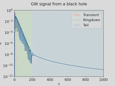
Either case, you get a gravitational wave signal that looks like this at infinity:

Why infinity? Infinity is the correct model for the wave signal because we observe gravitational waves from black holes that are hundreds of millions of light years away. That’s far. Very far. Mathematically, we model such distances by infinity, which we have wisely mapped to the outer boundary of our numerical domain. We’ve done it for technical reasons (to avoid numerical reflections, artificial truncation, to improve efficiency, etc.) but there are physical reasons why we’re interested in the data at infinity.

What you see in the signal above is a typical time evolution of a black-hole perturbation divided into three distinct phases: prompt response, exponential ringdown, and polynomial tail. This behavior has been studied for over half a century by now, yet we keep discovering new phenomena in the black-hole’s response to perturbations.

The prompt response is a transient phase triggered by the specifics of the perturbation. We used to discard this part because it depends on the initial data, but in the last 5 years or so there has been more attention to this piece in order to get a handle of the complete picture (see, for example, 2601.11706).

The ringdown is when the spacetime oscillates at a frequency that only depends on intrinsic properties of the black hole—in our case the mass. These characteristic modes are called quasinormal modes (QNMs). Intuitively, the energy from the perturbation absorbed by the black hole and escapes to infinity. Some of the energy that goes toward the black hole gets trapped by the photon sphere. This part becomes exponentially weaker with each cycle (see the above YouTube video) which we measure as QNM ringing. The hyperboloidal approach to QNMs has uncovered phenomena such as the pseudospectral instability that are active areas of research.

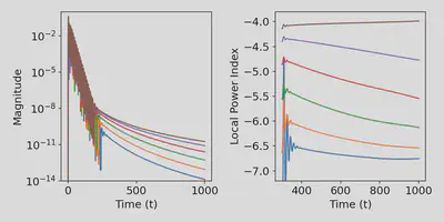
The part that escapes to infinity scatters off of the background curvature on its way and that scattered piece decays polynomially. It’s very weak, so it becomes only visible after the exponential ringdown becomes smaller than the polynomially decaying part. This part is also being studied currently, specifically the nonlinear tails. The plot on the right below shows the decay rates for observers at different distances from the black hole. For the $\ell=2$ perturbation, the infinity signal decays as $t^{-4}$ whereas the finite distance signal decays as $t^{-7}$.

Fading out

We just banged on a spacetime with a black hole and now you can create your own gravitational waves using a digital computer. Happy waving 👋